Tutorial¶

This is an introduction to LArray. It is not intended to be a fully comprehensive manual. It is mainly dedicated to help new users to familiarize with it and others to remind essentials.

The first step to use the LArray library is to import it:

In [1]: from larray import *

Axis creation¶

An axis represents a dimension of an LArray object. It consists of a name and a list of labels. They are several ways to create an axis:

# create a wildcard axis
In [2]: age = Axis(3, 'age')

# labels given as a list
In [3]: time = Axis([2007, 2008, 2009], 'time')

# create an axis using one string
In [4]: sex = Axis('sex=M,F')

# labels generated using a special syntax
In [5]: other = Axis('other=A01..C03')

In [6]: age, sex, time, other
Out[6]: 
(Axis(3, 'age'),
 Axis(['M', 'F'], 'sex'),
 Axis([2007, 2008, 2009], 'time'),
 Axis(['A01', 'A02', 'A03', 'B01', 'B02', 'B03', 'C01', 'C02', 'C03'], 'other'))

Array creation¶

A LArray object represents a multidimensional array with labeled axes.

From scratch¶

To create an array from scratch, you need to provide the data and a list of axes. Optionally, a title can be defined.

In [7]: import numpy as np

# list of the axes
In [8]: axes = [age, sex, time, other]

# data (the shape of data array must match axes lengths)
In [9]: data = np.random.randint(100, size=[len(axis) for axis in axes])

# title (optional)
In [10]: title = 'random data'

In [11]: arr = LArray(data, axes, title)

In [12]: arr
Out[12]: 
age*  sex  time\other  A01  A02  A03  B01  B02  B03  C01  C02  C03
   0    M        2007   11   26   93   57   75   82   45    2   13
   0    M        2008   55    9   50   76   33   91   38   25   69
   0    M        2009   53   28   72   40   30   69   35   24    7
   0    F        2007   38   60   34   41   23   51   55   83   78
   0    F        2008   23   81   60   31   88   78   85   16   43
   0    F        2009   69   63   92   48   34   69   51   61   18
   1    M        2007   17   37   86    9    3   58   88    9   41
   1    M        2008   15    4   74   47   23   81    8   25   15
   1    M        2009   36   30   63   27   35   34   93   31   86
   1    F        2007   50   18   86   95   79   46   76   11   39
   1    F        2008    2   99   11   97   24   18    1   27   23
   1    F        2009   70   59   13   82   80    6   39    6   88
   2    M        2007   61   74   81   57   34   66    9   42   79
   2    M        2008   23   67   29   58   77   43   29   74   49
   2    M        2009   85   46   44    4   74   17   64   34   95
   2    F        2007   18   98   29   62   86   43   19   12   65
   2    F        2008   28   87   32   91   22   51   40    4   38
   2    F        2009   41   76   97   97    5    3   45   58   40

Array creation functions¶

Arrays can also be generated in an easier way through creation functions:

ndrange() : fills an array with increasing numbers
ndtest() : same as ndrange but with axes generated automatically (for testing)
empty() : creates an array but leaves its allocated memory unchanged (i.e., it contains “garbage”. Be careful !)
zeros() : fills an array with 0
ones() : fills an array with 1
full() : fills an array with a given value

Except for ndtest, a list of axes must be provided. Axes can be passed in different ways:

as Axis objects
as integers defining the lengths of auto-generated wildcard axes
as a string : ‘sex=M,F;time=2007,2008,2009’ (name is optional)
as pairs (name, labels)

Optionally, the type of data stored by the array can be specified using argument dtype.

# start defines the starting value of data
In [13]: ndrange(['age=0..2', 'sex=M,F', 'time=2007..2009'], start=-1)
Out[13]: 
age  sex\time  2007  2008  2009
  0         M    -1     0     1
  0         F     2     3     4
  1         M     5     6     7
  1         F     8     9    10
  2         M    11    12    13
  2         F    14    15    16

# start defines the starting value of data
# label_start defines the starting index of labels
In [14]: ndtest((3, 3), start=-1, label_start=2)
Out[14]: 
a\b  b2  b3  b4
 a2  -1   0   1
 a3   2   3   4
 a4   5   6   7

# empty generates uninitialised array with correct axes (much faster but use with care!).
# This not really random either, it just reuses a portion of memory that is available, with whatever content is there.
# Use it only if performance matters and make sure all data will be overridden.
In [15]: empty(['age=0..2', 'sex=M,F', 'time=2007..2009'])
Out[15]: 
age  sex\time                   2007                    2008                    2009
  0         M   6.9180901376223e-310         2.84317546e-316   6.91809100536483e-310
  0         F  6.91806053025905e-310   6.91806051988683e-310                     0.0
  1         M                    0.0   6.91809100536483e-310                     0.0
  1         F                    0.0    6.9180660075894e-310   6.91809100536483e-310
  2         M                    0.0                     0.0   6.91809100536483e-310
  2         F   6.9180909566974e-310  2.865238098441256e+161  3.250037186622356e+178

# example with anonymous axes
In [16]: zeros(['0..2', 'M,F', '2007..2009'])
Out[16]: 
{0}  {1}\{2}  2007  2008  2009
  0        M   0.0   0.0   0.0
  0        F   0.0   0.0   0.0
  1        M   0.0   0.0   0.0
  1        F   0.0   0.0   0.0
  2        M   0.0   0.0   0.0
  2        F   0.0   0.0   0.0

# dtype=int forces to store int data instead of default float
In [17]: ones(['age=0..2', 'sex=M,F', 'time=2007..2009'], dtype=int)
Out[17]: 
age  sex\time  2007  2008  2009
  0         M     1     1     1
  0         F     1     1     1
  1         M     1     1     1
  1         F     1     1     1
  2         M     1     1     1
  2         F     1     1     1

In [18]: full(['age=0..2', 'sex=M,F', 'time=2007..2009'], 1.23)
Out[18]: 
age  sex\time  2007  2008  2009
  0         M  1.23  1.23  1.23
  0         F  1.23  1.23  1.23
  1         M  1.23  1.23  1.23
  1         F  1.23  1.23  1.23
  2         M  1.23  1.23  1.23
  2         F  1.23  1.23  1.23

All the above functions exist in {func}_like variants which take axes from another array

In [19]: ones_like(arr)
Out[19]: 
age*  sex  time\other  A01  A02  A03  B01  B02  B03  C01  C02  C03
  M        2007    1    1    1    1    1    1    1    1    1
  M        2008    1    1    1    1    1    1    1    1    1
  M        2009    1    1    1    1    1    1    1    1    1
  F        2007    1    1    1    1    1    1    1    1    1
  F        2008    1    1    1    1    1    1    1    1    1
  F        2009    1    1    1    1    1    1    1    1    1
  M        2007    1    1    1    1    1    1    1    1    1
  M        2008    1    1    1    1    1    1    1    1    1
  M        2009    1    1    1    1    1    1    1    1    1
  F        2007    1    1    1    1    1    1    1    1    1
  F        2008    1    1    1    1    1    1    1    1    1
  F        2009    1    1    1    1    1    1    1    1    1
  M        2007    1    1    1    1    1    1    1    1    1
  M        2008    1    1    1    1    1    1    1    1    1
  M        2009    1    1    1    1    1    1    1    1    1
  F        2007    1    1    1    1    1    1    1    1    1
  F        2008    1    1    1    1    1    1    1    1    1
  F        2009    1    1    1    1    1    1    1    1    1

Sequence¶

The special sequence() function allows you to create an array from an axis by iteratively applying a function to a given initial value. You can choose between inc and mult functions or define your own.

# With initial=1.0 and inc=0.5, we generate the sequence 1.0, 1.5, 2.0, 2.5, 3.0, ...
In [20]: sequence('sex=M,F', initial=1.0, inc=0.5)
Out[20]: 
sex    M    F
     1.0  1.5

# With initial=1.0 and mult=2.0, we generate the sequence 1.0, 2.0, 4.0, 8.0, ...
In [21]: sequence('age=0..2', initial=1.0, mult=2.0)
Out[21]: 
age    0    1    2
     1.0  2.0  4.0

# Using your own function
In [22]: sequence('time=2007..2009', initial=2.0, func=lambda value: value**2)
Out[22]: 
time  2007  2008  2009
       2.0   4.0  16.0

You can also create N-dimensional array by passing (N-1)-dimensional array to initial, inc or mult argument

In [23]: birth = LArray([1.05, 1.15], 'sex=M,F')

In [24]: cumulate_newborns = sequence('time=2007..2009', initial=0.0, inc=birth)

In [25]: cumulate_newborns
Out[25]: 
sex\time  2007  2008  2009
       M   0.0  1.05   2.1
       F   0.0  1.15   2.3

In [26]: initial = LArray([90, 100], 'sex=M,F')

In [27]: survival = LArray([0.96, 0.98], 'sex=M,F')

In [28]: pop = sequence('age=80..83', initial=initial, mult=survival)

In [29]: pop
Out[29]: 
sex\age     80                 81                 82                 83
      M   90.0  86.39999999999999             82.944           79.62624
      F  100.0               98.0  96.03999999999999  94.11919999999999

Load/Dump from files¶

Load from files¶

In [30]: example_dir = EXAMPLE_FILES_DIR

Arrays can be loaded from CSV files (see documentation of read_csv() for more details)

# read_tsv is a shortcut when data are separated by tabs instead of commas (default separator of read_csv)
# read_eurostat is a shortcut to read EUROSTAT TSV files
In [31]: household = read_csv(example_dir + 'hh.csv')

In [32]: household.info
Out[32]: 
26 x 3 x 7
 time [26]: 1991 1992 1993 ... 2014 2015 2016
 geo [3]: 'BruCap' 'Fla' 'Wal'
 hh_type [7]: 'SING' "'MAR0" 'MAR+' ... 'UNM+' 'H1P' 'OTHR'
dtype: int64

or Excel sheets (see documentation of read_excel() for more details)

# loads array from the first sheet if no sheetname is given
In [33]: pop = read_excel(example_dir + 'demography.xlsx', 'pop')

In [34]: pop.info
Out[34]: 
26 x 3 x 121 x 2 x 2
 time [26]: 1991 1992 1993 ... 2014 2015 2016
 geo [3]: 'BruCap' 'Fla' 'Wal'
 age [121]: 0 1 2 ... 118 119 120
 sex [2]: 'M' 'F'
 nat [2]: 'BE' 'FO'
dtype: int64

or HDF5 files (HDF5 is file format designed to store and organize large amounts of data. An HDF5 file can contain multiple arrays. See documentation of read_hdf() for more details)

In [35]: mortality = read_hdf(example_dir + 'demography.h5','qx')

In [36]: mortality.info
Out[36]: 
26 x 3 x 121 x 2 x 2
 time [26]: 1991 1992 1993 ... 2014 2015 2016
 geo [3]: 'BruCap' 'Fla' 'Wal'
 age [121]: 0 1 2 ... 118 119 120
 sex [2]: 'M' 'F'
 nat [2]: 'BE' 'FO'
dtype: float64

Dump in files¶

Arrays can be dumped in CSV files (see documentation of to_csv() for more details)

In [37]: household.to_csv('hh2.csv')

or in Excel files (see documentation of to_excel() for more details)

 # if the file does not already exist, it is created with a single sheet,
 # otherwise a new sheet is added to it
In [38]: household.to_excel('demography_2.xlsx', overwrite_file=True)

 # it is usually better to specify the sheet explicitly (by name or position) though
In [39]: household.to_excel('demography_2.xlsx', 'hh')

or in HDF5 files (see documentation of to_hdf() for more details)

In [40]: household.to_hdf('demography_2.h5', 'hh')

more Excel IO¶

# create a 3 x 2 x 3 array
In [41]: age, sex, time = Axis('age=0..2'), Axis('sex=M,F'), Axis('time=2007..2009')

In [42]: arr = ndrange([age, sex, time])

In [43]: arr
Out[43]: 
age  sex\time  2007  2008  2009
  0         M     0     1     2
  0         F     3     4     5
  1         M     6     7     8
  1         F     9    10    11
  2         M    12    13    14
  2         F    15    16    17

Write Arrays¶

Open an Excel file

In [44]: wb = open_excel('test.xlsx', overwrite_file=True)

Put an array in an Excel Sheet, excluding headers (labels)

 # put arr at A1 in Sheet1, excluding headers (labels)
In [45]: wb['Sheet1'] = arr

 # same but starting at A9
 # note that Sheet1 must exist
In [46]: wb['Sheet1']['A9'] = arr

Put an array in an Excel Sheet, including headers (labels)

 # dump arr at A1 in Sheet2, including headers (labels)
In [47]: wb['Sheet2'] = arr.dump()

 # same but starting at A10
In [48]: wb['Sheet2']['A10'] = arr.dump()

Save file to disk

In [49]: wb.save()

Close file

In [50]: wb.close()

Read Arrays¶

Open an Excel file

In [51]: wb = open_excel('test.xlsx')

Load an array from a sheet (assuming the presence of (correctly formatted) headers and only one array in sheet)

# save one array in Sheet3 (including headers)
In [52]: wb['Sheet3'] = arr.dump()

# load array from the data starting at A1 in Sheet3
In [53]: arr = wb['Sheet3'].load()

In [54]: arr
Out[54]: 
age  sex\time  2007  2008  2009
  0         M     0     1     2
  0         F     3     4     5
  1         M     6     7     8
  1         F     9    10    11
  2         M    12    13    14
  2         F    15    16    17

Load an array with its axes information from a range

# if you need to use the same sheet several times,
# you can create a sheet variable
In [55]: sheet2 = wb['Sheet2']

# load array contained in the 4 x 4 table defined by cells A10 and D14
In [56]: arr2 = sheet2['A10:D14'].load()

In [57]: arr2
Out[57]: 
age  sex\time  2007  2008
  0         M     0     1
  0         F     3     4
  1         M     6     7
  1         F     9    10

Read Ranges (experimental)¶

Load an array (raw data) with no axis information from a range

In [58]: arr3 = wb['Sheet1']['A1:B4']

In [59]: arr3
Out[59]: 
{0}*\{1}*  0   1
        0  0   1
        1  3   4
        2  6   7
        3  9  10

in fact, this is not really an LArray …

In [60]: type(arr3)
larray.io.excel.Range

… but it can be used as such

In [61]: arr3.sum(axis=0)
Out[61]: 
{0}*   0   1
      18  22

… and it can be used for other stuff, like setting the formula instead of the value:

In [62]: arr3.formula = '=D10+1'

In the future, we should also be able to set font name, size, style, etc.

In [63]: wb.close()

Inspecting¶

# load population array
In [64]: pop = load_example_data('demography').pop

Get array summary : dimensions + description of axes

In [65]: pop.info
Out[65]: 
26 x 3 x 121 x 2 x 2
 time [26]: 1991 1992 1993 ... 2014 2015 2016
 geo [3]: 'BruCap' 'Fla' 'Wal'
 age [121]: 0 1 2 ... 118 119 120
 sex [2]: 'M' 'F'
 nat [2]: 'BE' 'FO'
dtype: int64

Get axes

In [66]: time, geo, age, sex, nat = pop.axes

Get array dimensions

In [67]: pop.shape
Out[67]: (26, 3, 121, 2, 2)

Get number of elements

In [68]: pop.size
Out[68]: 37752

Get size in memory

In [69]: pop.nbytes
Out[69]: 302016

Start viewer (graphical user interface) in read-only mode. This will open a new window and block execution of the rest of code until the windows is closed! Required PyQt installed.

In [70]: view(pop)

Load array in an Excel sheet

In [71]: pop.to_excel()

Selection (Subsets)¶

LArray allows to select a subset of an array either by labels or positions

Selection by Labels¶

To take a subset of an array using labels, use brackets [ ]. Let’s start by selecting a single element:

# here we select the value associated with Belgian women of age 50 from Brussels region for the year 2015
In [72]: pop[2015, 'BruCap', 50, 'F', 'BE']
Out[72]: 4813

Continue with selecting a subset using slices and lists of labels

# here we select the subset associated with Belgian women of age 50, 51 and 52
# from Brussels region for the years 2010 to 2016
In [73]: pop[2010:2016, 'BruCap', 50:52, 'F', 'BE']
Out[73]: 
time\age    50    51    52
    2010  4869  4811  4699
    2011  5015  4860  4792
    2012  4722  5014  4818
    2013  4711  4727  5007
    2014  4788  4702  4730
    2015  4813  4767  4676
    2016  4814  4792  4740

# slices bounds are optional:
# if not given start is assumed to be the first label and stop is the last one.
# Here we select all years starting from 2010
In [74]: pop[2010:, 'BruCap', 50:52, 'F', 'BE']
Out[74]: 
time\age    50    51    52
    2010  4869  4811  4699
    2011  5015  4860  4792
    2012  4722  5014  4818
    2013  4711  4727  5007
    2014  4788  4702  4730
    2015  4813  4767  4676
    2016  4814  4792  4740

# Slices can also have a step (defaults to 1), to take every Nth labels
# Here we select all even years starting from 2010
In [75]: pop[2010::2, 'BruCap', 50:52, 'F', 'BE']
Out[75]: 
time\age    50    51    52
    2010  4869  4811  4699
    2012  4722  5014  4818
    2014  4788  4702  4730
    2016  4814  4792  4740

# one can also use list of labels to take non-contiguous labels.
# Here we select years 2008, 2010, 2013 and 2015
In [76]: pop[[2008, 2010, 2013, 2015], 'BruCap', 50:52, 'F', 'BE']
Out[76]: 
time\age    50    51    52
    2008  4731  4735  4724
    2010  4869  4811  4699
    2013  4711  4727  5007
    2015  4813  4767  4676

The order of indexing does not matter either, so you usually do not care/have to remember about axes positions during computation. It only matters for output.

# order of index doesn't matter
In [77]: pop['F', 'BE', 'BruCap', [2008, 2010, 2013, 2015], 50:52]
Out[77]: 
time\age    50    51    52
    2008  4731  4735  4724
    2010  4869  4811  4699
    2013  4711  4727  5007
    2015  4813  4767  4676

Warning

Selecting by labels as above works well as long as there is no ambiguity. When two or more axes have common labels, it may lead to a crash. The solution is then to precise to which axis belong the labels.

# let us now create an array with the same labels on several axes
In [78]: age, weight, size = Axis('age=0..80'), Axis('weight=0..120'), Axis('size=0..200')

In [79]: arr_ws = ndrange([age, weight, size])

# let's try to select teenagers with size between 1 m 60 and 1 m 65 and weight > 80 kg.
# In this case the subset is ambiguous and this results in an error:
In [80]: arr_ws[10:18, :80, 160:165]
<class 'ValueError'> slice(10, 18, None) is ambiguous (valid in age, weight, size)

# the solution is simple. You need to precise the axes on which you make a selection
In [81]: arr_ws[age[10:18], weight[:80], size[160:165]]
Out[81]: 
age  weight\size     160     161     162     163     164     165
 10            0  243370  243371  243372  243373  243374  243375
 10            1  243571  243572  243573  243574  243575  243576
 10            2  243772  243773  243774  243775  243776  243777
 10            3  243973  243974  243975  243976  243977  243978
 10            4  244174  244175  244176  244177  244178  244179
...          ...     ...     ...     ...     ...     ...     ...
 18           76  453214  453215  453216  453217  453218  453219
 18           77  453415  453416  453417  453418  453419  453420
 18           78  453616  453617  453618  453619  453620  453621
 18           79  453817  453818  453819  453820  453821  453822
 18           80  454018  454019  454020  454021  454022  454023

Special variable x¶

When selecting, assiging or using aggregate functions, an axis can be refered via the special variable x:

pop[x.age[:20]]
pop.sum(x.age)

This gives you acces to axes of the array you are manipulating. The main drawback of using x is that you lose the autocompletion available from many editors. It only works with non-wildcard axes.

# the previous example could have been also written as
In [82]: arr_ws[x.age[10:18], x.weight[:80], x.size[160:165]]
Out[82]: 
age  weight\size     160     161     162     163     164     165
 10            0  243370  243371  243372  243373  243374  243375
 10            1  243571  243572  243573  243574  243575  243576
 10            2  243772  243773  243774  243775  243776  243777
 10            3  243973  243974  243975  243976  243977  243978
 10            4  244174  244175  244176  244177  244178  244179
...          ...     ...     ...     ...     ...     ...     ...
 18           76  453214  453215  453216  453217  453218  453219
 18           77  453415  453416  453417  453418  453419  453420
 18           78  453616  453617  453618  453619  453620  453621
 18           79  453817  453818  453819  453820  453821  453822
 18           80  454018  454019  454020  454021  454022  454023

Selection by Positions¶

Sometimes it is more practical to use positions along the axis, instead of labels. You need to add the character i before the brackets: .i[positions]. As for selection with labels, you can use single position or slice or list of positions. Positions can be also negative (-1 represent the last element of an axis).

Note

Remember that positions (indices) are always 0-based in Python. So the first element is at position 0, the second is at position 1, etc.

# here we select the subset associated with Belgian women of age 50, 51 and 52
# from Brussels region for the first 3 years
In [83]: pop[x.time.i[:3], 'BruCap', 50:52, 'F', 'BE']
Out[83]: 
time\age    50    51    52
    1991  3739  4138  4101
    1992  3373  3665  4088
    1993  3648  3335  3615

# same but for the last 3 years
In [84]: pop[x.time.i[-3:], 'BruCap', 50:52, 'F', 'BE']
Out[84]: 
time\age    50    51    52
    2014  4788  4702  4730
    2015  4813  4767  4676
    2016  4814  4792  4740

# using list of positions
In [85]: pop[x.time.i[-9,-7,-4,-2], 'BruCap', 50:52, 'F', 'BE']
Out[85]: 
time\age    50    51    52
    2008  4731  4735  4724
    2010  4869  4811  4699
    2013  4711  4727  5007
    2015  4813  4767  4676

Warning

The end indice (position) is EXCLUSIVE while the end label is INCLUSIVE.

# with labels (3 is included)
In [86]: pop[2015, 'BruCap', x.age[:3], 'F', 'BE']
Out[86]: 
age     0     1     2     3
     6020  5882  6023  5861

# with position (3 is out)
In [87]: pop[2015, 'BruCap', x.age.i[:3], 'F', 'BE']
Out[87]: 
age     0     1     2
     6020  5882  6023

You can use .i[] selection directly on array instead of axes. In this context, if you want to select a subset of the first and third axes for example, you must use a full slice : for the second one.

# here we select the last year and first 3 ages
# equivalent to: pop.i[-1, :, :3, :, :]
In [88]: pop.i[-1, :, :3]
Out[88]: 
   geo  age  sex\nat     BE    FO
BruCap    0        M   6155  3104
BruCap    0        F   5900  2817
BruCap    1        M   6165  3068
BruCap    1        F   5916  2946
BruCap    2        M   6053  2918
BruCap    2        F   5736  2776
   Fla    0        M  29993  3717
   Fla    0        F  28483  3587
   Fla    1        M  31292  3716
   Fla    1        F  29721  3575
   Fla    2        M  31718  3597
   Fla    2        F  30353  3387
   Wal    0        M  17869  1472
   Wal    0        F  17242  1454
   Wal    1        M  18820  1432
   Wal    1        F  17604  1443
   Wal    2        M  19076  1444
   Wal    2        F  18189  1358

Assigning subsets¶

Assigning value¶

Assign a value to a subset

# let's take a smaller array
In [89]: pop = load_example_data('demography').pop[2016, 'BruCap', 100:105]

In [90]: pop2 = pop

In [91]: pop2
Out[91]: 
age  sex\nat  BE  FO
100        M  12   0
100        F  60   3
101        M  12   2
101        F  66   5
102        M   8   0
102        F  26   1
103        M   2   1
103        F  17   2
104        M   2   1
104        F  14   0
105        M   0   0
105        F   2   2

# set all data corresponding to age >= 102 to 0
In [92]: pop2[102:] = 0

In [93]: pop2
Out[93]: 
age  sex\nat  BE  FO
      M  12   0
      F  60   3
      M  12   2
      F  66   5
      M   0   0
      F   0   0
      M   0   0
      F   0   0
      M   0   0
      F   0   0
      M   0   0
      F   0   0

One very important gotcha though…

Warning

Modifying a slice of an array in-place like we did above should be done with care otherwise you could have unexpected effects. The reason is that taking a slice subset of an array does not return a copy of that array, but rather a view on that array. To avoid such behavior, use .copy() method.

Remember:

taking a slice subset of an array is extremely fast (no data is copied)
if one modifies that subset in-place, one also modifies the original array
.copy() returns a copy of the subset (takes speed and memory) but allows you to change the subset without modifying the original array in the same time

# indeed, data from the original array have also changed
In [94]: pop
Out[94]: 
age  sex\nat  BE  FO
      M  12   0
      F  60   3
      M  12   2
      F  66   5
      M   0   0
      F   0   0
      M   0   0
      F   0   0
      M   0   0
      F   0   0
      M   0   0
      F   0   0

# the right way
In [95]: pop = load_example_data('demography').pop[2016, 'BruCap', 100:105]

In [96]: pop2 = pop.copy()

In [97]: pop2[102:] = 0

In [98]: pop2
Out[98]: 
age  sex\nat  BE  FO
100        M  12   0
100        F  60   3
101        M  12   2
101        F  66   5
102        M   0   0
102        F   0   0
103        M   0   0
103        F   0   0
104        M   0   0
104        F   0   0
105        M   0   0
105        F   0   0

# now, data from the original array have not changed this time
In [99]: pop
Out[99]: 
age  sex\nat  BE  FO
      M  12   0
      F  60   3
      M  12   2
      F  66   5
      M   8   0
      F  26   1
      M   2   1
      F  17   2
      M   2   1
      F  14   0
      M   0   0
      F   2   2

Assigning Arrays & Broadcasting¶

Instead of a value, we can also assign an array to a subset. In that case, that array can have less axes than the target but those which are present must be compatible with the subset being targeted.

In [100]: sex, nat = Axis('sex=M,F'), Axis('nat=BE,FO')

In [101]: new_value = LArray([[1, -1], [2, -2]],[sex, nat])

In [102]: new_value
Out[102]: 
sex\nat  BE  FO
      M   1  -1
      F   2  -2

# this assigns 1, -1 to Belgian, Foreigner men
# and 2, -2 to Belgian, Foreigner women for all
# people older than 100
In [103]: pop[102:] = new_value

In [104]: pop
Out[104]: 
age  sex\nat  BE  FO
100        M  12   0
100        F  60   3
101        M  12   2
101        F  66   5
102        M   1  -1
102        F   2  -2
103        M   1  -1
103        F   2  -2
104        M   1  -1
104        F   2  -2
105        M   1  -1
105        F   2  -2

Warning

The array being assigned must have compatible axes with the target subset.

# assume we define the following array with shape 3 x 2 x 2
In [105]: new_value = zeros(['age=0..2', sex, nat])

In [106]: new_value
Out[106]: 
age  sex\nat   BE   FO
  0        M  0.0  0.0
  0        F  0.0  0.0
  1        M  0.0  0.0
  1        F  0.0  0.0
  2        M  0.0  0.0
  2        F  0.0  0.0

# now let's try to assign the previous array in a subset with shape 7 x 2 x 2
In [107]: pop[102:] = new_value
<class 'ValueError'> could not broadcast input array from shape (3,2,2) into shape (4,2,2)

# but this works
In [108]: pop[102:104] = new_value
---------------------------------------------------------------------------
ValueError                                Traceback (most recent call last)
<ipython-input-108-182e038e029c> in <module>()
----> 1 pop[102:104] = new_value

~/checkouts/readthedocs.org/user_builds/larray-test/conda/stable/lib/python3.5/site-packages/larray-0.27-py3.5.egg/larray/core/array.py in __setitem__(self, key, value, collapse_slices)
   2168                 axes = self._get_axes_from_translated_key(translated_key)
   2169             value = value.broadcast_with(axes)
-> 2170             value.axes.check_compatible(axes)
   2171 
   2172             # replace incomprehensible error message "could not broadcast input array from shape XX into shape YY"

~/checkouts/readthedocs.org/user_builds/larray-test/conda/stable/lib/python3.5/site-packages/larray-0.27-py3.5.egg/larray/core/axis.py in check_compatible(self, axes)
   1713             local_axis = self.get_by_pos(axis, i)
   1714             if not local_axis.iscompatible(axis):
-> 1715                 raise ValueError("incompatible axes:\n{!r}\nvs\n{!r}".format(axis, local_axis))
   1716 
   1717     def extend(self, axes, validate=True, replace_wildcards=False):

ValueError: incompatible axes:
Axis([102, 103, 104], 'age')
vs
Axis([0, 1, 2], 'age')

In [109]: pop
Out[109]: 
age  sex\nat  BE  FO
100        M  12   0
100        F  60   3
101        M  12   2
101        F  66   5
102        M   1  -1
102        F   2  -2
103        M   1  -1
103        F   2  -2
104        M   1  -1
104        F   2  -2
105        M   1  -1
105        F   2  -2

Boolean filtering¶

Boolean filtering can be use to extract subsets.

#Let's focus on population living in Brussels during the year 2016
In [110]: pop = load_example_data('demography').pop[2016, 'BruCap']

# here we select all males and females with age less than 5 and 10 respectively
In [111]: subset = pop[((x.sex == 'H') & (x.age <= 5)) | ((x.sex == 'F') & (x.age <= 10))]

In [112]: subset
Out[112]: 
age_sex\nat    BE    FO
        0_F  5900  2817
        1_F  5916  2946
        2_F  5736  2776
        3_F  5883  2734
        4_F  5784  2523
        5_F  5780  2521
        6_F  5759  2290
        7_F  5518  2234
        8_F  5474  2066
        9_F  5354  1896
       10_F  5200  1785

Note

Be aware that after boolean filtering, several axes may have merged.

# 'age' and 'sex' axes have been merged together
In [113]: subset.info
Out[113]: 
11 x 2
 age_sex [11]: '0_F' '1_F' '2_F' ... '8_F' '9_F' '10_F'
 nat [2]: 'BE' 'FO'
dtype: int64

This may be not what you because previous selections on merged axes are no longer valid

# now let's try to calculate the proportion of females with age less than 10
In [114]: subset['F'].sum() / pop['F'].sum()
<class 'ValueError'> F is not a valid label for any axis

Therefore, it is sometimes more useful to not select, but rather set to 0 (or another value) non matching elements

In [115]: subset = pop.copy()

In [116]: subset[((x.sex == 'F') & (x.age > 10))] = 0

In [117]: subset['F', :20]
Out[117]: 
age\nat    BE    FO
5900  2817
5916  2946
5736  2776
5883  2734
5784  2523
5780  2521
5759  2290
5518  2234
5474  2066
5354  1896
5200  1785
   0     0
   0     0
   0     0
   0     0
   0     0
   0     0
   0     0
   0     0
   0     0
   0     0

# now we can calculate the proportion of females with age less than 10
In [118]: subset['F'].sum() / pop['F'].sum()
Out[118]: 0.14618110657051941

Boolean filtering can also mix axes and arrays. Example above could also have been written as

In [119]: age_limit = sequence('sex=M,F', initial=5, inc=5)

In [120]: age_limit
Out[120]: 
sex  M   F
     5  10

In [121]: age = pop.axes['age']

In [122]: (age <= age_limit)[:20]
Out[122]: 
age\sex      M      F
 True   True
 True   True
 True   True
 True   True
 True   True
 True   True
False   True
False   True
False   True
False   True
False   True
False  False
False  False
False  False
False  False
False  False
False  False
False  False
False  False
False  False
False  False

In [123]: subset = pop.copy()

In [124]: subset[x.age > age_limit] = 0

In [125]: subset['F'].sum() / pop['F'].sum()
Out[125]: 0.14618110657051941

Finally, you can choose to filter on data instead of axes

# let's focus on females older than 90
In [126]: subset = pop['F', 90:110].copy()

In [127]: subset
Out[127]: 
age\nat    BE   FO
1477  136
1298  105
1141   78
 906   74
 739   65
 566   53
 327   25
 171   21
 135    9
  92    8
  60    3
  66    5
  26    1
  17    2
  14    0
   2    2
   3    3
   1    2
   1    0
   0    0
   0    0

# here we set to 0 all data < 10
In [128]: subset[subset < 10] = 0

In [129]: subset
Out[129]: 
age\nat    BE   FO
1477  136
1298  105
1141   78
 906   74
 739   65
 566   53
 327   25
 171   21
 135    0
  92    0
  60    0
  66    0
  26    0
  17    0
  14    0
   0    0
   0    0
   0    0
   0    0
   0    0
   0    0

Manipulates axes from arrays¶

# let's start with
In [130]: pop = load_example_data('demography').pop[2016, 'BruCap', 90:95]

In [131]: pop
Out[131]: 
age  sex\nat    BE   FO
      M   539   74
      F  1477  136
      M   499   49
      F  1298  105
      M   332   35
      F  1141   78
      M   287   27
      F   906   74
      M   237   23
      F   739   65
      M   154   19
      F   566   53

Relabeling¶

Replace all labels of one axis

# returns a copy by default
In [132]: pop_new_labels = pop.set_labels(x.sex, ['Men', 'Women'])

In [133]: pop_new_labels
Out[133]: 
age  sex\nat    BE   FO
    Men   539   74
  Women  1477  136
    Men   499   49
  Women  1298  105
    Men   332   35
  Women  1141   78
    Men   287   27
  Women   906   74
    Men   237   23
  Women   739   65
    Men   154   19
  Women   566   53

# inplace flag avoids to create a copy
In [134]: pop.set_labels(x.sex, ['M', 'F'], inplace=True)
Out[134]: 
age  sex\nat    BE   FO
      M   539   74
      F  1477  136
      M   499   49
      F  1298  105
      M   332   35
      F  1141   78
      M   287   27
      F   906   74
      M   237   23
      F   739   65
      M   154   19
      F   566   53

Renaming axes¶

Rename one axis

In [135]: pop.info
Out[135]: 
6 x 2 x 2
 age [6]: 90 91 92 93 94 95
 sex [2]: 'M' 'F'
 nat [2]: 'BE' 'FO'
dtype: int64

# 'rename' returns a copy of the array
In [136]: pop2 = pop.rename(x.sex, 'gender')

In [137]: pop2
Out[137]: 
age  gender\nat    BE   FO
         M   539   74
         F  1477  136
         M   499   49
         F  1298  105
         M   332   35
         F  1141   78
         M   287   27
         F   906   74
         M   237   23
         F   739   65
         M   154   19
         F   566   53

Rename several axes at once

# No x. here because sex and nat are keywords and not actual axes
In [138]: pop2 = pop.rename(sex='gender', nat='nationality')

In [139]: pop2
Out[139]: 
age  gender\nationality    BE   FO
                 M   539   74
                 F  1477  136
                 M   499   49
                 F  1298  105
                 M   332   35
                 F  1141   78
                 M   287   27
                 F   906   74
                 M   237   23
                 F   739   65
                 M   154   19
                 F   566   53

Reordering axes¶

Axes can be reordered using transpose() method. By default, transpose reverse axes, otherwise it permutes the axes according to the list given as argument. Axes not mentioned come after those which are mentioned(and keep their relative order). Finally, transpose returns a copy of the array.

# starting order : age, sex, nat
In [140]: pop
Out[140]: 
age  sex\nat    BE   FO
      M   539   74
      F  1477  136
      M   499   49
      F  1298  105
      M   332   35
      F  1141   78
      M   287   27
      F   906   74
      M   237   23
      F   739   65
      M   154   19
      F   566   53

# no argument --> reverse axes
In [141]: pop.transpose()
Out[141]: 
nat  sex\age    90    91    92   93   94   95
 BE        M   539   499   332  287  237  154
 BE        F  1477  1298  1141  906  739  566
 FO        M    74    49    35   27   23   19
 FO        F   136   105    78   74   65   53

# .T is a shortcut for .transpose()
In [142]: pop.T
Out[142]: 
nat  sex\age    90    91    92   93   94   95
 BE        M   539   499   332  287  237  154
 BE        F  1477  1298  1141  906  739  566
 FO        M    74    49    35   27   23   19
 FO        F   136   105    78   74   65   53

# reorder according to list
In [143]: pop.transpose(x.age, x.nat, x.sex)
Out[143]: 
age  nat\sex    M     F
     BE  539  1477
     FO   74   136
     BE  499  1298
     FO   49   105
     BE  332  1141
     FO   35    78
     BE  287   906
     FO   27    74
     BE  237   739
     FO   23    65
     BE  154   566
     FO   19    53

# axes not mentioned come after those which are mentioned (and keep their relative order)
In [144]: pop.transpose(x.sex)
Out[144]: 
sex  age\nat    BE   FO
  M       90   539   74
  M       91   499   49
  M       92   332   35
  M       93   287   27
  M       94   237   23
  M       95   154   19
  F       90  1477  136
  F       91  1298  105
  F       92  1141   78
  F       93   906   74
  F       94   739   65
  F       95   566   53

Aggregates¶

Calculate the sum along an axis

In [145]: pop = load_example_data('demography').pop[2016, 'BruCap']

In [146]: pop.sum(x.age)
Out[146]: 
sex\nat      BE      FO
      M  375261  204534
      F  401554  206541

or along all axes except one by appending _by to the aggregation function

In [147]: pop[90:95].sum_by(x.age)
Out[147]: 
age    90    91    92    93    94   95
     2226  1951  1586  1294  1064  792

# is equivalent to
In [148]: pop[90:95].sum(x.sex, x.nat)
Out[148]: 
age    90    91    92    93    94   95
     2226  1951  1586  1294  1064  792

There are many other aggregate functions built-in:

mean, min, max, median, percentile, var (variance), std (standard deviation)
labelofmin, labelofmax (label indirect minimum/maxium – labels where the value is minimum/maximum)
indexofmin, indexofmax (positional indirect minimum/maxium – position along axis where the value is minimum/maximum)
cumsum, cumprod (cumulative sum, cumulative product)

Groups¶

One can define groups of labels (or indices)

In [149]: age = pop.axes['age']

# using indices (remember: 20 will not be included)
In [150]: teens = age.i[10:20]

# using labels
In [151]: pensioners = age[67:]

In [152]: strange = age[[30, 55, 52, 25, 99]]

In [153]: strange
Out[153]: age[30, 55, 52, 25, 99]

or rename them

# method 'named' returns a new group with the given name
In [154]: teens = teens.named('children')

# operator >> is a shortcut for 'named'
In [155]: pensioners = pensioners >> 'pensioners'

In [156]: pensioners
Out[156]: age[67:] >> 'pensioners'

Then, use them in selections

In [157]: pop[strange]
Out[157]: 
age  sex\nat    BE    FO
      M  5278  4725
      F  5253  5419
      M  4457  2196
      F  4953  2059
      M  4635  2640
      F  4740  2333
      M  5477  3590
      F  5539  4635
      M    20     2
      F    92     8

or aggregations

In [158]: pop.sum(pensioners)
Out[158]: 
sex\nat     BE     FO
      M  44138   9939
      F  70314  13241

# several groups (here you see the interest of groups renaming)
In [159]: pop.sum((teens, pensioners, strange))
Out[159]: 
           age  sex\nat     BE     FO
      children        M  49143  17100
      children        F  47226  16523
    pensioners        M  44138   9939
    pensioners        F  70314  13241
30,55,52,25,99        M  19867  13153
30,55,52,25,99        F  20577  14454

# combined with other axes
In [160]: pop.sum((teens, pensioners, strange), x.nat)
Out[160]: 
       age\sex      M      F
      children  66243  63749
    pensioners  54077  83555
30,55,52,25,99  33020  35031

Arithmetic operations¶

# go back to our 6 x 2 x 2 example array
In [161]: pop = load_example_data('demography').pop[2016, 'BruCap', 90:95]

In [162]: pop
Out[162]: 
age  sex\nat    BE   FO
      M   539   74
      F  1477  136
      M   499   49
      F  1298  105
      M   332   35
      F  1141   78
      M   287   27
      F   906   74
      M   237   23
      F   739   65
      M   154   19
      F   566   53

Usual Operations¶

One can do all usual arithmetic operations on an array, it will apply the operation to all elements individually

# addition
In [163]: pop + 200
Out[163]: 
age  sex\nat    BE   FO
      M   739  274
      F  1677  336
      M   699  249
      F  1498  305
      M   532  235
      F  1341  278
      M   487  227
      F  1106  274
      M   437  223
      F   939  265
      M   354  219
      F   766  253

# multiplication
In [164]: pop * 2
Out[164]: 
age  sex\nat    BE   FO
      M  1078  148
      F  2954  272
      M   998   98
      F  2596  210
      M   664   70
      F  2282  156
      M   574   54
      F  1812  148
      M   474   46
      F  1478  130
      M   308   38
      F  1132  106

# ** means raising to the power (squaring in this case)
In [165]: pop ** 2
Out[165]: 
age  sex\nat       BE     FO
      M   290521   5476
      F  2181529  18496
      M   249001   2401
      F  1684804  11025
      M   110224   1225
      F  1301881   6084
      M    82369    729
      F   820836   5476
      M    56169    529
      F   546121   4225
      M    23716    361
      F   320356   2809

# % means modulo (aka remainder of division)
In [166]: pop % 10
Out[166]: 
age  sex\nat  BE  FO
      M   9   4
      F   7   6
      M   9   9
      F   8   5
      M   2   5
      F   1   8
      M   7   7
      F   6   4
      M   7   3
      F   9   5
      M   4   9
      F   6   3

More interestingly, it also works between two arrays

# load mortality equivalent array
In [167]: mortality = load_example_data('demography').qx[2016, 'BruCap', 90:95]

# compute number of deaths
In [168]: death = pop * mortality

In [169]: death
Out[169]: 
age  sex\nat                  BE                  FO
 90        M   94.00000000000001  13.000000000000004
 90        F  204.00000000000003  19.000000000000004
 91        M                95.0                 9.0
 91        F  200.00000000000006                16.0
 92        M                70.0                 7.0
 92        F  195.00000000000006  13.000000000000004
 93        M   66.00000000000001                 6.0
 93        F  171.99999999999997                14.0
 94        M                59.0                 6.0
 94        F  155.00000000000003                14.0
 95        M                41.0                 5.0
 95        F               130.0  12.000000000000004

Note

Be careful when mixing different data types. See type promotion in programming. You can use the method astype() to change the data type of an array.

# to be sure to get number of deaths as integers
# one can use .astype() method
In [170]: death = (pop * mortality).astype(int)

In [171]: death
Out[171]: 
age  sex\nat   BE  FO
 90        M   94  13
 90        F  204  19
 91        M   95   9
 91        F  200  16
 92        M   70   7
 92        F  195  13
 93        M   66   6
 93        F  171  14
 94        M   59   6
 94        F  155  14
 95        M   41   5
 95        F  130  12

But operations between two arrays only works when they have compatible axes (i.e. same labels)

In [172]: pop[90:92] * mortality[93:95]
<class 'ValueError'> incompatible axes:
Axis([93, 94, 95], 'age')
vs
Axis([90, 91, 92], 'age')

You can override that but at your own risk. In that case only the position on the axis is used and not the labels.

In [173]: pop[90:92] * mortality[93:95].drop_labels(x.age)
Out[173]: 
age  sex\nat                  BE                  FO
 90        M  123.95121951219514  16.444444444444443
 90        F    280.401766004415   25.72972972972973
 91        M  124.22362869198312  12.782608695652174
 91        F  272.24627875507446  22.615384615384617
 92        M   88.38961038961038   9.210526315789473
 92        F  262.06713780918733   17.66037735849057

Boolean Operations¶

In [174]: pop2 = pop.copy()

In [175]: pop2['F'] = -pop2['F']

In [176]: pop2
Out[176]: 
age  sex\nat     BE    FO
      M    539    74
      F  -1477  -136
      M    499    49
      F  -1298  -105
      M    332    35
      F  -1141   -78
      M    287    27
      F   -906   -74
      M    237    23
      F   -739   -65
      M    154    19
      F   -566   -53

# testing for equality is done using == (a single = assigns the value)
In [177]: pop == pop2
Out[177]: 
age  sex\nat     BE     FO
      M   True   True
      F  False  False
      M   True   True
      F  False  False
      M   True   True
      F  False  False
      M   True   True
      F  False  False
      M   True   True
      F  False  False
      M   True   True
      F  False  False

# testing for inequality
In [178]: pop != pop2
Out[178]: 
age  sex\nat     BE     FO
      M  False  False
      F   True   True
      M  False  False
      F   True   True
      M  False  False
      F   True   True
      M  False  False
      F   True   True
      M  False  False
      F   True   True
      M  False  False
      F   True   True

# what was our original array like again?
In [179]: pop
Out[179]: 
age  sex\nat    BE   FO
      M   539   74
      F  1477  136
      M   499   49
      F  1298  105
      M   332   35
      F  1141   78
      M   287   27
      F   906   74
      M   237   23
      F   739   65
      M   154   19
      F   566   53

# & means (boolean array) and
In [180]: (pop >= 500) & (pop <= 1000)
Out[180]: 
age  sex\nat     BE     FO
      M   True  False
      F  False  False
      M  False  False
      F  False  False
      M  False  False
      F  False  False
      M  False  False
      F   True  False
      M  False  False
      F   True  False
      M  False  False
      F   True  False

# | means (boolean array) or
In [181]: (pop < 500) | (pop > 1000)
Out[181]: 
age  sex\nat     BE    FO
      M  False  True
      F   True  True
      M   True  True
      F   True  True
      M   True  True
      F   True  True
      M   True  True
      F  False  True
      M   True  True
      F  False  True
      M   True  True
      F  False  True

Arithmetic operations with missing axes¶

In [182]: pop.sum(x.age)
Out[182]: 
sex\nat    BE   FO
      M  2048  227
      F  6127  511

# arr has 3 dimensions
In [183]: pop.info
Out[183]: 
6 x 2 x 2
 age [6]: 90 91 92 93 94 95
 sex [2]: 'M' 'F'
 nat [2]: 'BE' 'FO'
dtype: int64

# and arr.sum(age) has two
In [184]: pop.sum(x.age).info
Out[184]: 
2 x 2
 sex [2]: 'M' 'F'
 nat [2]: 'BE' 'FO'
dtype: int64

# you can do operation with missing axes so this works
In [185]: pop / pop.sum(x.age)
Out[185]: 
age  sex\nat                   BE                   FO
      M        0.26318359375  0.32599118942731276
      F   0.2410641423208748  0.26614481409001955
      M        0.24365234375  0.21585903083700442
      F   0.2118491921005386   0.2054794520547945
      M          0.162109375  0.15418502202643172
      F  0.18622490615309287  0.15264187866927592
      M        0.14013671875  0.11894273127753303
      F  0.14787008323812634  0.14481409001956946
      M        0.11572265625   0.1013215859030837
      F  0.12061367716663947  0.12720156555772993
      M         0.0751953125  0.08370044052863436
      F  0.09237799902072792  0.10371819960861056

Axis order does not matter much (except for output)¶

You can do operations between arrays having different axes order. The axis order of the result is the same as the left array

In [186]: pop
Out[186]: 
age  sex\nat    BE   FO
      M   539   74
      F  1477  136
      M   499   49
      F  1298  105
      M   332   35
      F  1141   78
      M   287   27
      F   906   74
      M   237   23
      F   739   65
      M   154   19
      F   566   53

# let us change the order of axes
In [187]: pop_transposed = pop.T

In [188]: pop_transposed
Out[188]: 
nat  sex\age    90    91    92   93   94   95
 BE        M   539   499   332  287  237  154
 BE        F  1477  1298  1141  906  739  566
 FO        M    74    49    35   27   23   19
 FO        F   136   105    78   74   65   53

# mind blowing
In [189]: pop_transposed + pop
Out[189]: 
nat  sex\age    90    91    92    93    94    95
 BE        M  1078   998   664   574   474   308
 BE        F  2954  2596  2282  1812  1478  1132
 FO        M   148    98    70    54    46    38
 FO        F   272   210   156   148   130   106

Combining arrays¶

Append/Prepend¶

Append/prepend one element to an axis of an array

In [190]: pop = load_example_data('demography').pop[2016, 'BruCap', 90:95]

# imagine that you have now acces to the number of non-EU foreigners
In [191]: data = [[25, 54], [15, 33], [12, 28], [11, 37], [5, 21], [7, 19]]

In [192]: pop_non_eu = LArray(data, pop['FO'].axes)

# you can do something like this
In [193]: pop = pop.append(nat, pop_non_eu, 'NEU')

In [194]: pop
Out[194]: 
age  sex\nat    BE   FO  NEU
 90        M   539   74   25
 90        F  1477  136   54
 91        M   499   49   15
 91        F  1298  105   33
 92        M   332   35   12
 92        F  1141   78   28
 93        M   287   27   11
 93        F   906   74   37
 94        M   237   23    5
 94        F   739   65   21
 95        M   154   19    7
 95        F   566   53   19

# you can also add something at the start of an axis
In [195]: pop = pop.prepend(x.sex, pop.sum(x.sex), 'B')

In [196]: pop
Out[196]: 
age  sex\nat    BE   FO  NEU
      B  2016  210   79
      M   539   74   25
      F  1477  136   54
      B  1797  154   48
      M   499   49   15
      F  1298  105   33
      B  1473  113   40
      M   332   35   12
      F  1141   78   28
      B  1193  101   48
      M   287   27   11
      F   906   74   37
      B   976   88   26
      M   237   23    5
      F   739   65   21
      B   720   72   26
      M   154   19    7
      F   566   53   19

The value being appended/prepended can have missing (or even extra) axes as long as common axes are compatible

In [197]: aliens = zeros(pop.axes['sex'])

In [198]: aliens
Out[198]: 
sex    B    M    F
     0.0  0.0  0.0

In [199]: pop = pop.append(x.nat, aliens, 'AL')

In [200]: pop
Out[200]: 
age  sex\nat      BE     FO   NEU   AL
      B  2016.0  210.0  79.0  0.0
      M   539.0   74.0  25.0  0.0
      F  1477.0  136.0  54.0  0.0
      B  1797.0  154.0  48.0  0.0
      M   499.0   49.0  15.0  0.0
      F  1298.0  105.0  33.0  0.0
      B  1473.0  113.0  40.0  0.0
      M   332.0   35.0  12.0  0.0
      F  1141.0   78.0  28.0  0.0
      B  1193.0  101.0  48.0  0.0
      M   287.0   27.0  11.0  0.0
      F   906.0   74.0  37.0  0.0
      B   976.0   88.0  26.0  0.0
      M   237.0   23.0   5.0  0.0
      F   739.0   65.0  21.0  0.0
      B   720.0   72.0  26.0  0.0
      M   154.0   19.0   7.0  0.0
      F   566.0   53.0  19.0  0.0

Extend¶

Extend an array along an axis with another array with that axis (but other labels)

In [201]: _pop = load_example_data('demography').pop

In [202]: pop = _pop[2016, 'BruCap', 90:95]

In [203]: pop_next = _pop[2016, 'BruCap', 96:100]

# concatenate along age axis
In [204]: pop.extend(x.age, pop_next)
Out[204]: 
age  sex\nat    BE   FO
      M   539   74
      F  1477  136
      M   499   49
      F  1298  105
      M   332   35
      F  1141   78
      M   287   27
      F   906   74
      M   237   23
      F   739   65
      M   154   19
      F   566   53
      M    80    9
      F   327   25
      M    43    9
      F   171   21
      M    23    4
      F   135    9
      M    20    2
      F    92    8
      M    12    0
      F    60    3

Stack¶

Stack several arrays together to create an entirely new dimension

# imagine you have loaded data for each nationality in different arrays (e.g. loaded from different Excel sheets)
In [205]: pop_be, pop_fo = pop['BE'], pop['FO']

# first way to stack them
In [206]: nat = Axis('nat=BE,FO,NEU')

In [207]: pop = stack([pop_be, pop_fo, pop_non_eu], nat)

# second way
In [208]: pop = stack([('BE', pop_be), ('FO', pop_fo), ('NEU', pop_non_eu)], 'nat')

In [209]: pop
Out[209]: 
age  sex\nat    BE   FO  NEU
 90        M   539   74   25
 90        F  1477  136   54
 91        M   499   49   15
 91        F  1298  105   33
 92        M   332   35   12
 92        F  1141   78   28
 93        M   287   27   11
 93        F   906   74   37
 94        M   237   23    5
 94        F   739   65   21
 95        M   154   19    7
 95        F   566   53   19

Sorting¶

Sort an axis (alphabetically if labels are strings)

In [210]: pop_sorted = pop.sort_axes(x.nat)

In [211]: pop_sorted
Out[211]: 
age  sex\nat    BE   FO  NEU
      M   539   74   25
      F  1477  136   54
      M   499   49   15
      F  1298  105   33
      M   332   35   12
      F  1141   78   28
      M   287   27   11
      F   906   74   37
      M   237   23    5
      F   739   65   21
      M   154   19    7
      F   566   53   19

Give labels which would sort the axis

In [212]: pop_sorted.labelsofsorted(x.sex)
Out[212]: 
age  sex\nat  BE  FO  NEU
      0   M   M    M
      1   F   F    F
      0   M   M    M
      1   F   F    F
      0   M   M    M
      1   F   F    F
      0   M   M    M
      1   F   F    F
      0   M   M    M
      1   F   F    F
      0   M   M    M
      1   F   F    F

Sort according to values

In [213]: pop_sorted.sort_values((90, 'F'))
Out[213]: 
age  sex\nat  NEU   FO    BE
      M   25   74   539
      F   54  136  1477
      M   15   49   499
      F   33  105  1298
      M   12   35   332
      F   28   78  1141
      M   11   27   287
      F   37   74   906
      M    5   23   237
      F   21   65   739
      M    7   19   154
      F   19   53   566

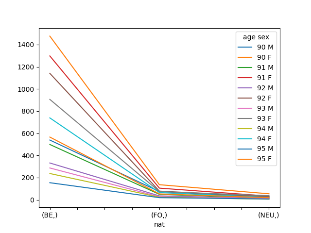
Plotting¶

Create a plot (last axis define the different curves to draw)

In [214]: pop.plot()
Out[214]: <matplotlib.axes._subplots.AxesSubplot at 0x7f59ab5966d8>

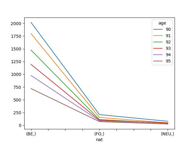
# plot total of both sex
In [215]: pop.sum(x.sex).plot()
Out[215]: <matplotlib.axes._subplots.AxesSubplot at 0x7f59ab426f60>

Interesting methods¶

# starting array
In [216]: pop = load_example_data('demography').pop[2016, 'BruCap', 100:105]

In [217]: pop
Out[217]: 
age  sex\nat  BE  FO
      M  12   0
      F  60   3
      M  12   2
      F  66   5
      M   8   0
      F  26   1
      M   2   1
      F  17   2
      M   2   1
      F  14   0
      M   0   0
      F   2   2

with total¶

Add totals to one axis

In [218]: pop.with_total(x.sex, label='B')
Out[218]: 
age  sex\nat  BE  FO
      M  12   0
      F  60   3
      B  72   3
      M  12   2
      F  66   5
      B  78   7
      M   8   0
      F  26   1
      B  34   1
      M   2   1
      F  17   2
      B  19   3
      M   2   1
      F  14   0
      B  16   1
      M   0   0
      F   2   2
      B   2   2

Add totals to all axes at once

# by default label is 'total'
In [219]: pop.with_total()
Out[219]: 
  age  sex\nat   BE  FO  total
      M   12   0     12
      F   60   3     63
  total   72   3     75
      M   12   2     14
      F   66   5     71
  total   78   7     85
      M    8   0      8
      F   26   1     27
  total   34   1     35
      M    2   1      3
      F   17   2     19
  total   19   3     22
      M    2   1      3
      F   14   0     14
  total   16   1     17
      M    0   0      0
      F    2   2      4
  total    2   2      4
total        M   36   4     40
total        F  185  13    198
total    total  221  17    238

where¶

where can be used to apply some computation depending on a condition

# where(condition, value if true, value if false)
In [220]: where(pop < 10, 0, -pop)
Out[220]: 
age  sex\nat   BE  FO
      M  -12   0
      F  -60   0
      M  -12   0
      F  -66   0
      M    0   0
      F  -26   0
      M    0   0
      F  -17   0
      M    0   0
      F  -14   0
      M    0   0
      F    0   0

clip¶

Set all data between a certain range

# clip(min, max)
# values below 10 are set to 10 and values above 50 are set to 50
In [221]: pop.clip(10, 50)
Out[221]: 
age  sex\nat  BE  FO
      M  12  10
      F  50  10
      M  12  10
      F  50  10
      M  10  10
      F  26  10
      M  10  10
      F  17  10
      M  10  10
      F  14  10
      M  10  10
      F  10  10

divnot0¶

Replace division by 0 to 0

In [222]: pop['BE'] / pop['FO']
Out[222]: 
age\sex    M     F
    100  inf  20.0
    101  6.0  13.2
    102  inf  26.0
    103  2.0   8.5
    104  2.0   inf
    105  nan   1.0

# divnot0 replaces results of division by 0 by 0.
# Using it should be done with care though
# because it can hide a real error in your data.
In [223]: pop['BE'].divnot0(pop['FO'])
Out[223]: 
age\sex    M     F
    100  0.0  20.0
    101  6.0  13.2
    102  0.0  26.0
    103  2.0   8.5
    104  2.0   0.0
    105  0.0   1.0

diff¶

diff() calculates the n-th order discrete difference along given axis. The first order difference is given by out[n+1] = in[n + 1] - in[n] along the given axis.

In [224]: pop = load_example_data('demography').pop[2005:2015, 'BruCap', 50]

In [225]: pop
Out[225]: 
time  sex\nat    BE    FO
      M  4289  1591
      F  4661  1584
      M  4335  1761
      F  4781  1580
      M  4291  1806
      F  4719  1650
      M  4349  1773
      F  4731  1680
      M  4429  2003
      F  4824  1722
      M  4582  2085
      F  4869  1928
      M  4677  2294
      F  5015  2104
      M  4463  2450
      F  4722  2186
      M  4610  2604
      F  4711  2254
      M  4725  2709
      F  4788  2349
      M  4841  2891
      F  4813  2498

# calculates 'pop[year+1] - pop[year]'
In [226]: pop.diff(x.time)
Out[226]: 
time  sex\nat    BE   FO
      M    46  170
      F   120   -4
      M   -44   45
      F   -62   70
      M    58  -33
      F    12   30
      M    80  230
      F    93   42
      M   153   82
      F    45  206
      M    95  209
      F   146  176
      M  -214  156
      F  -293   82
      M   147  154
      F   -11   68
      M   115  105
      F    77   95
      M   116  182
      F    25  149

# calculates 'pop[year+2] - pop[year]'
In [227]: pop.diff(x.time, d=2)
Out[227]: 
time  sex\nat    BE   FO
      M     2  215
      F    58   66
      M    14   12
      F   -50  100
      M   138  197
      F   105   72
      M   233  312
      F   138  248
      M   248  291
      F   191  382
      M  -119  365
      F  -147  258
      M   -67  310
      F  -304  150
      M   262  259
      F    66  163
      M   231  287
      F   102  244

ratio¶

In [228]: pop.ratio(x.nat)
Out[228]: 
time  sex\nat                  BE                   FO
      M   0.729421768707483    0.270578231292517
      F  0.7463570856685349   0.2536429143314652
      M  0.7111220472440944   0.2888779527559055
      F  0.7516113818581984   0.2483886181418016
      M   0.703788748564868  0.29621125143513205
      F  0.7409326424870466  0.25906735751295334
      M  0.7103887618425351  0.28961123815746487
      F  0.7379503977538605  0.26204960224613943
      M  0.6885883084577115  0.31141169154228854
      F  0.7369385884509624  0.26306141154903756
      M  0.6872656367181641   0.3127343632818359
      F  0.7163454465205238   0.2836545534794762
      M  0.6709223927700474  0.32907760722995266
      F  0.7044528725944655  0.29554712740553446
      M  0.6455952553160712  0.35440474468392885
      F  0.6835552982049797  0.31644470179502027
      M  0.6390352093152204   0.3609647906847796
      F  0.6763819095477387   0.3236180904522613
      M   0.635593220338983   0.3644067796610169
      F  0.6708701134930644   0.3291298865069357
      M  0.6260993274702535   0.3739006725297465
      F  0.6583230748187663  0.34167692518123377

# which is equivalent to
In [229]: pop / pop.sum(x.nat)
Out[229]: 
time  sex\nat                  BE                   FO
      M   0.729421768707483    0.270578231292517
      F  0.7463570856685349   0.2536429143314652
      M  0.7111220472440944   0.2888779527559055
      F  0.7516113818581984   0.2483886181418016
      M   0.703788748564868  0.29621125143513205
      F  0.7409326424870466  0.25906735751295334
      M  0.7103887618425351  0.28961123815746487
      F  0.7379503977538605  0.26204960224613943
      M  0.6885883084577115  0.31141169154228854
      F  0.7369385884509624  0.26306141154903756
      M  0.6872656367181641   0.3127343632818359
      F  0.7163454465205238   0.2836545534794762
      M  0.6709223927700474  0.32907760722995266
      F  0.7044528725944655  0.29554712740553446
      M  0.6455952553160712  0.35440474468392885
      F  0.6835552982049797  0.31644470179502027
      M  0.6390352093152204   0.3609647906847796
      F  0.6763819095477387   0.3236180904522613
      M   0.635593220338983   0.3644067796610169
      F  0.6708701134930644   0.3291298865069357
      M  0.6260993274702535   0.3739006725297465
      F  0.6583230748187663  0.34167692518123377

percents¶

# or, if you want the previous ratios in percents
In [230]: pop.percent(x.nat)
Out[230]: 
time  sex\nat                  BE                  FO
      M    72.9421768707483    27.0578231292517
      F   74.63570856685348  25.364291433146516
      M   71.11220472440945  28.887795275590552
      F   75.16113818581984   24.83886181418016
      M    70.3788748564868  29.621125143513204
      F   74.09326424870466  25.906735751295336
      M   71.03887618425351   28.96112381574649
      F   73.79503977538606  26.204960224613945
      M   68.85883084577114  31.141169154228855
      F   73.69385884509624   26.30614115490376
      M   68.72656367181641  31.273436328183593
      F   71.63454465205237  28.365455347947623
      M   67.09223927700474   32.90776072299526
      F   70.44528725944654  29.554712740553448
      M   64.55952553160712  35.440474468392885
      F   68.35552982049798  31.644470179502026
      M   63.90352093152204   36.09647906847796
      F   67.63819095477388   32.36180904522613
      M  63.559322033898304  36.440677966101696
      F   67.08701134930644   32.91298865069357
      M   62.60993274702535   37.39006725297465
      F   65.83230748187663  34.167692518123374

growth_rate¶

using the same principle than diff…

In [231]: pop.growth_rate(x.time)
Out[231]: 
time  sex\nat                     BE                      FO
      M   0.010725110748426206     0.10685103708359522
      F   0.025745548165629694  -0.0025252525252525255
      M  -0.010149942329873126     0.02555366269165247
      F  -0.012967998326709893     0.04430379746835443
      M   0.013516662782568165   -0.018272425249169437
      F  0.0025429116338207248     0.01818181818181818
      M    0.01839503334099793     0.12972363226170333
      F   0.019657577679137603                   0.025
      M    0.03454504402799729    0.040938592111832255
      F   0.009328358208955223     0.11962833914053426
      M    0.02073330423395897     0.10023980815347722
      F   0.029985623331279524      0.0912863070539419
      M   -0.04575582638443447     0.06800348735832606
      F    -0.0584247258225324     0.03897338403041825
      M    0.03293748599596684     0.06285714285714286
      F  -0.002329521389241847     0.03110704483074108
      M   0.024945770065075923     0.04032258064516129
      F    0.01634472511144131     0.04214729370008873
      M    0.02455026455026455     0.06718346253229975
      F  0.0052213868003341685     0.06343124733929331

shift¶

The shift() method drops first label of an axis and shifts all subsequent labels

In [232]: pop.shift(x.time)
Out[232]: 
time  sex\nat    BE    FO
      M  4289  1591
      F  4661  1584
      M  4335  1761
      F  4781  1580
      M  4291  1806
      F  4719  1650
      M  4349  1773
      F  4731  1680
      M  4429  2003
      F  4824  1722
      M  4582  2085
      F  4869  1928
      M  4677  2294
      F  5015  2104
      M  4463  2450
      F  4722  2186
      M  4610  2604
      F  4711  2254
      M  4725  2709
      F  4788  2349

# when shift is applied on an (increasing) time axis, it effectively brings "past" data into the future
In [233]: pop.shift(x.time).drop_labels(x.time) == pop[2005:2014].drop_labels(x.time)
Out[233]: 
time*  sex\nat    BE    FO
      M  True  True
      F  True  True
      M  True  True
      F  True  True
      M  True  True
      F  True  True
      M  True  True
      F  True  True
      M  True  True
      F  True  True
      M  True  True
      F  True  True
      M  True  True
      F  True  True
      M  True  True
      F  True  True
      M  True  True
      F  True  True
      M  True  True
      F  True  True

# this is mostly useful when you want to do operations between the past and now
# as an example, here is an alternative implementation of the .diff method seen above:
In [234]: pop.i[1:] - pop.shift(x.time)
Out[234]: 
time  sex\nat    BE   FO
      M    46  170
      F   120   -4
      M   -44   45
      F   -62   70
      M    58  -33
      F    12   30
      M    80  230
      F    93   42
      M   153   82
      F    45  206
      M    95  209
      F   146  176
      M  -214  156
      F  -293   82
      M   147  154
      F   -11   68
      M   115  105
      F    77   95
      M   116  182
      F    25  149

Misc other interesting functions¶

There are a lot more functions available:

round, floor, ceil, trunc,
exp, log, log10,
sqrt, absolute, nan_to_num, isnan, isinf, inverse,
sin, cos, tan, arcsin, arccos, arctan
and many many more…

Sessions¶

You can group several arrays in a Session

# load several arrays
In [235]: arr1, arr2, arr3 = ndtest((3, 3)), ndtest((4, 2)), ndtest((2, 4))

# create and populate a 'session'
In [236]: s1 = Session()

In [237]: s1.arr1 = arr1

In [238]: s1.arr2 = arr2

In [239]: s1.arr3 = arr3

In [240]: s1
Out[240]: Session(arr1, arr2, arr3)

The advantage of sessions is that you can manipulate all of the arrays in them in one shot

# this saves all the arrays in a single excel file (each array on a different sheet)
In [241]: s1.save('test.xlsx')

# this saves all the arrays in a single HDF5 file (which is a very fast format)
In [242]: s1.save('test.h5')

# this creates a session out of all arrays in the .h5 file
In [243]: s2 = Session('test.h5')

In [244]: s2
Out[244]: Session(arr1, arr2, arr3)

# this creates a session out of all arrays in the .xlsx file
In [245]: s3 = Session('test.xlsx')

In [246]: s3
Out[246]: Session(arr1, arr2, arr3)

You can compare two sessions

In [247]: s1 == s2
Out[247]: 
name  arr1  arr2  arr3
      True  True  True

# let us introduce a difference (a variant, or a mistake perhaps)
In [248]: s2.arr1['a0', 'b1':] = 0

In [249]: s1 == s2
Out[249]: 
name   arr1  arr2  arr3
      False  True  True

In [250]: s1_diff = s1[s1 != s2]

In [251]: s1_diff
Out[251]: Session(arr1)

In [252]: s2_diff = s2[s1 != s2]

In [253]: s2_diff
Out[253]: Session(arr1)

This a bit experimental but can be useful nonetheless (Open a graphical interface)

In [254]: compare(s1_diff.arr1, s2_diff.arr1)